


LTspice tips 'n tricks
Here you will find some tips for beginners on LTspice: LTspice is a free (and one of the best, too!) SPICE simulator developed in-house by Linear Technologies, one of the leading semiconductor companies, now part of Analog Devices.
For a very good wiki, with lots of good info, articles, examples on LTspice, visit ltwiki.org; in particular have a look at the
FAQ section.
Index
- Hotkeys
- Add a model to a symbol
- Copy a schematic to another page
- Create a symbol from a device model
- Sanity check of simulation results
- Import and export data
- Generate a complex transfer function using a behavioural source
- Generate a triangular or a sawtooth waveform
- Examples using the .MEASURE statement
- Simulate a pushbutton press using a voltage controlled switch
- Simulate a time-varying resistance value
- Step trough component values using the .STEP statement
- Set initial conditions
- Mathematical & Logical operators list
- Save a node voltage or current as .wav audio file using the .WAVE statement
- Attach the cursor in the Waveform Viewer window to a specific run (e.g. when using the .STEP statement)
Hotkeys
from the flyer on Analog Devices website
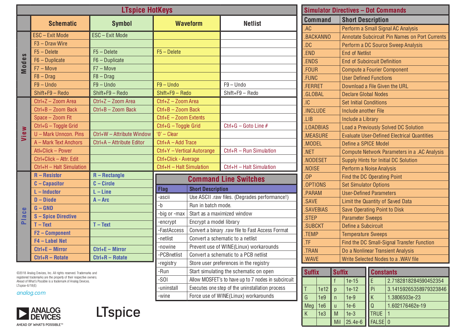
Other LTspice Key combinations:
Shift+Ctrl+Alt+R: Renumbers all reference designators in the schematic
Shift+Ctrl+Alt+H: Highlights all hidden text in the schematic
Hold down Ctrl when placing wires to route at any angle
Hold down Ctrl when drawing lines to draw off grid
Hold down Ctrl or Shift for more travel with the arrow keys
Hold down Ctrl and Shift for most travel with the arrow keys
Text preceeded with an underscore "_" will have an OVERBAR (useful to label "active low" digital signals)
Add a model to a symbol
In order to simulate a specific device (e.g. an OPA381 opamp) you have to point LTspice to a simulation model, a text file describing the device. You generally download these from the manufacturer website. Some examples:
OPA381.LIB is the model file for the OPA381 opamp from Texas Instruments.
HSMS-258x.LIB is the model file for the HSMS-258x diode from Agilent.
To create a simulation library file from scratch, using the SPICE parameters found in some datasheets, you can use the library files above as a template to modify with the paramaters you are given in the datasheet, checking the correspondence between the parameters names used in the datasheet and those used in LTspice, using the pdf manual from Analog Devices or the online manual at ltwiki.org (look inside the Circuit Elements section for the name and description of every parameter used by each LTspice primitive - diode, resistor, mosfet, etc).
There are two types of third-party SPICE models, those described with a .MODEL statement and those described with the .SUBCKT statement:
- models using the .MODEL statement are used for intrinsic SPICE devices (aka primitive), like diodes and transistors: the behaviour is already defined in SPICE and the model adds
only the parameters' values, defining the specific electrical characteristics of the device. - models using the .SUBCKT statement defines component modeled using circuits made with multiple SPICE primitives: an opamp is defined as a subcircuit using this statement.
Example for a component defined with the .MODEL statement: npn transistor
- Start by designing the circuit: use the symbol NPN for the transistor
- Copy the library file containing the model for the bjt, for instance Bipolar.lib in the same directory of the schematic
- Add the SPICE directive .INCLUDE Bipolar.lib to the schematic (press S) , or you can paste the file contents directly in the schematic page using a multi-line text box
- Right click on the component (for some components like transistors you need to also press the AltGr key when right-clicking, otherwise it will only let you choose the transistor model from a predefined list) and modify the value field from "NPN" to the name in the .MODEL statement in the library file (you can open it with LTspice or any text editor), in this case "BC547C".
Do not change the Prefix attribute.
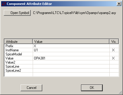
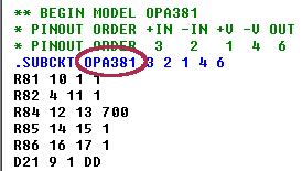
Example for a component defined with the .SUBCKT statement: operational amplifier
- Start by designing the circuit: use the symbol opamp2 for the opamp
- Copy the library file OPA381.LIB in the same directory of the schematic
- Add the SPICE directive .INCLUDE OPA381.LIB to the schematic (press S) , or you can paste the file contents directly in the schematic page using a multi-line text box
- Right click on the component (for some components like transistors you need to also press the AltGr key when right-clicking, otherwise it will only let you choose the transistor model from a predefined list) and modify the value field from "opamp2" to the name in the .SUBCKT statement in the library file (you can open it with LTspice or any text editor), in this case "OPA381".
Also change the Prefix attribute to X.
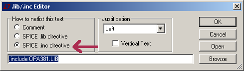
NOTES:
If using a .SUBCKT model make sure that the model and the symbol have the same pin/port netlist order.
If you get an the error message like "Unknown subcircuit called in: x1 n003 n009 n011 OPA381", make sure that the "include" statement is marked as spice .inc directive and not as Comment (see the image below), otherwise you probably did not write correctly the name of the model file in the statement.

Copy a schematic to another page
Open the two pages: both have to be visible so you need to reduce one window to a smaller size. Then use the copy command (<F6> key) to copy from one page to the other.
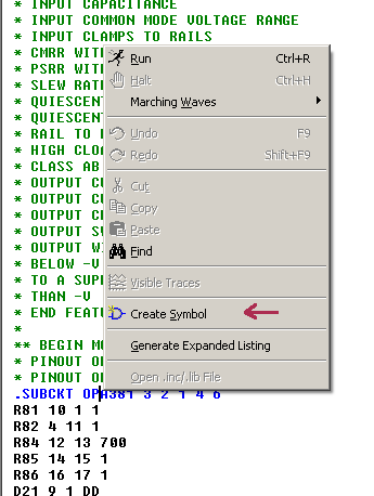
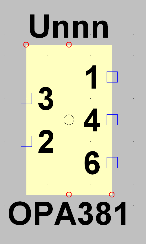
Create a symbol from a device model
Open the model file in LTspice, move the mouse cursor over the .SUBCKT statement and right clickand select Create Symbol: it will be created a square symbol having all the pins of the model. The symbol will be created in a directory called AutoGenerated inside the symbols directory, for instance: C:\Programs\LTspiceIV\lib\sym\AutoGenerated.
Sanity check of simulation results
You may want to check that all currents, voltages of a simulation have 'safe' values:
The Octave/Matlab script ltspice.sanity.check.m prints the minimum, maximum, RMS value for each simulation variable (any voltage, current, power) previously saved in a text file from whitin LTspice.
First download the Octave/Matlab script ltspice.sanity.check.m
Then perform a simulation with LTspice, and save the simulation results with File -> Export and select the traces you want to check (see Import and export data below).
Then you need to convert the tab-separated values file to a comma-separated values one using the Linux BASH script tsv2csv.sh.
From the shell prompt execute:
$ ./tsv2csv.sh <NOMEfile>
you will also need my Octave/Matlab function StampaSettori.m to print the data nicely in columns.
In ltspice.sanity.check.m you also need to modify the line data_array=csv2cell('NOMEFILE.tsv.csv') with your file name , and finally execute the script.
Import and export data
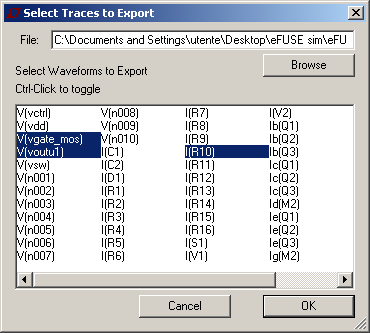
To export waveform data to an ACSII text file:
- Click on the waveform viewer to select it (or open a .raw file containing the waveforms you want to save)
- Click on File -> Export (this menu is only visible if the waveform viewer window is selected)
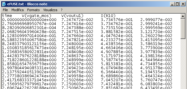
- Select the traces (waveforms) you want to export and click OK
The waveform will be saved in a .txt file having the same name of the schematic
note: in a large simulation you may want to limit the .raw output file (which is always generated by LTspice) size by telliong LTspice to only save some specific voltages and current waveforms, using the following dot command:
.SAVE V(Vout1) V(Vin) ..etc
To use an externally generated waveform into LTspice you must use a voltage or current source and configure it to use an input file in the piecewise linear (PWL) function section
The input file must contain a list of values that represent time-value data pairs in a tab or comma separated format.
The PWL function builds a waveform based on linear interpolation between the points defined in the text file.
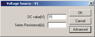
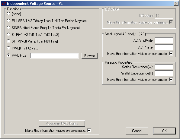
To add a text file as a PWL function to a voltage or current source:
- In the schematic editor right-click the voltage or current generator symbol
- Click on the Advanced button
- In the Functions section select PWL FILE and click on the Browse button to choose the text file
Generate a complex transfer function using a behavioural source
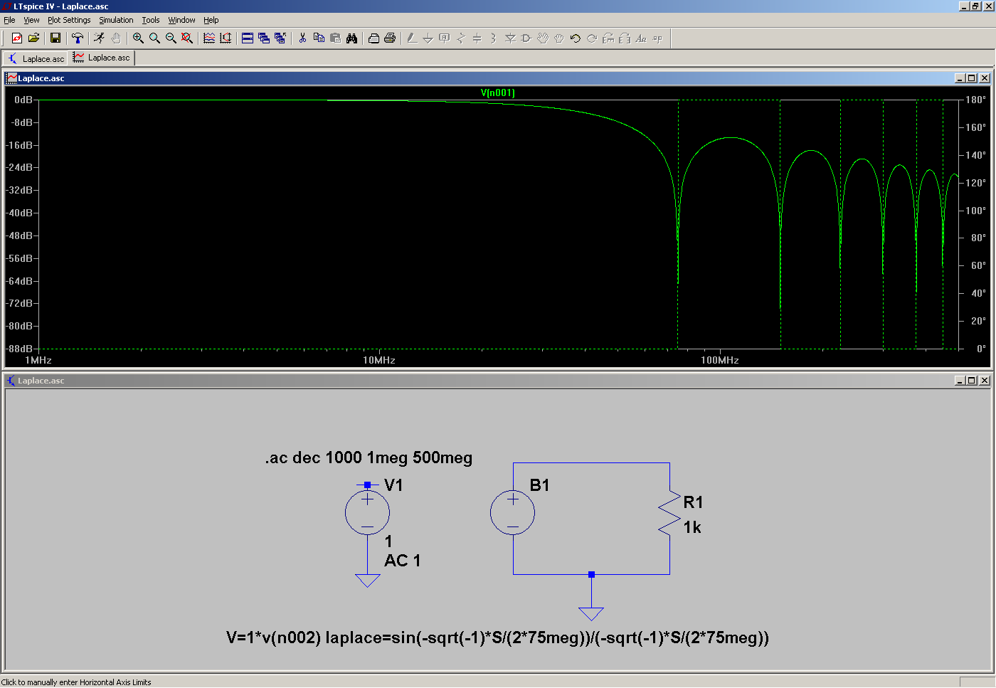
I used a behavioural voltage source to simulate a zero-order-hold sinc() envelope transfer function in the frequency domain (.AC analysis) from the output DAC of a Direct Digital Synthesis IC: this was needed to simulate the transfer function (in the frequency domain) of the DAC and the following lowpass filter.
B1 transfer function (converted to the frequency domain using the Laplace transform) is:
sinc(π f / Fs) = sin (-i / (2 Fs)) / (-i / (2 Fs)),
where S= i 2π f, i is the imaginary unit and Fs is the DDS IC's internal DAC sampling frequency.
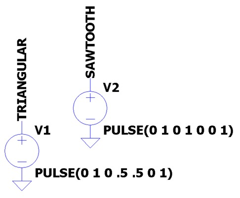
Generate a triangular or a sawtooth waveform
Use the PULSE function of an independent voltage or current source to generate a triangular or a sawtooth wave
Syntax:
PULSE(Voff Von Tdelay Trise Tfall Ton Tperiod Ncycles)
For a triangular waveform set the rise and fall time equal to half the period, for a sawtooth fuction set the rise time equal to the period and the fall time to zero
[image from http://www.linear.com/solutions/LTspice]
Examples using the .MEASURE statement
Syntax:
.MEAS [AC|DC|OP|TRAN|TF|NOISE] <name>
+
[<AVG|MAX|MIN|PP|RMS|INTEG> <expr>]
+ [TRIG <lhs1> [[VAL]=]<rhs1>] [TD=<val1>]
+
[<RISE|FALL|CROSS>=<count1>]
+ [TARG <lhs2> [[VAL]=]<rhs2>] [TD=<val2>]
+
[<RISE|FALL|CROSS>=<count2>]
NOTES:
The simulation type (AC, DC, ...) is optional and it is used to execute a .MEAS statement only with a certain simulation type.
giving a name with <name> allows to use the result of a .MEAS statement in a following .MEAS statement.
The output of this command is written in the "Error Log" file (<PROJECT_NAME>.log) which can be viewed by clicking on: View -> SPICE Error Log.
If the simulation includes a .STEP command, the .MEAS statements are executed for each step and can be plotted like normal waveforms by opening right click in the .log file and choosing "Plot .step'ed .meas data".
Print the value of the voltage at the "out" node at t=10ms and label it "result"
.MEAS TRAN result FIND V(out) AT=10m
Print the value of V(out) the third time the condition V(x)=5*V(y) is true
.MEAS TRAN result FIND V(out) WHEN V(x)=5*V(y) cross=3
Print the frequency at which the magnitude of V(out) is equal to 1/√2
.MEAS AC f_pole when V(out)=1/sqrt(2)
Print the RMS value of the voltage at node "out"
.MEAS Vrms RMS V(out)
Print the average value of the voltage at node "out"
.MEAS Vaverage AVG V(out)
(You can also use MAX, MIN, PP to calculate the maximum, minimum and peak-to-peak value respectively)
Print the difference between the two previously calculated values (param is needed to use the results of a previous instance of .MEASURE)
.MEAS DELTA param (Vrms-Vaverage)
Print the -3dB bandwidth on a passband circuit: find the peak response and call it "Vpk", then calculate the difference in frequency between the two points 3dB down from peak response.
.MEAS AC Vpk MAX MAG(V(out))
.MEAS AC BandWidth TRIG MAG(V(out))=Vpk/sqrt(2) RISE=1 TARG MAG(V(out))=Vpk/sqrt(2) FALL=last
Simulate a pushbutton press using a voltage controlled switch
I used a voltage controlled switch to simulate someone pressing a pushbutton, used in this case to reset a circuit.
PULSE(0 1 5 1m) means that the 0V -> 1V pulse happens at t=5s and the risetime is equal to 1 ms
Remember to right click on the switch and modify the value field from "SW" to the name in the .MODEL statement ("MySwitch" in my example).

Simulate a time-varying resistance value
To vary a resistance over time during a .TRAN simulation (e.g. to simulate a time-varying load):
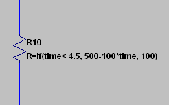
right click onto an existing resistor, and enter a formula like:
R=20-100*time
to vary a resistor from 20Ω to 10Ω in 100ms
To avoid negative resistance values use something like:
R=if(time<100m, 20-100*time, 10)
The resistance value will still drop from 20 to 10Ω in 100 ms but from then on the resistance will remain 10Ω
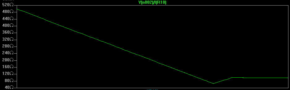
In the example below (a TRAN simulation) the resistance value is first decreased from 500Ω to 50Ω in 4.5 seconds, then its value is set to 100Ω: note that the resistance linearly increases to the final value and does not vary instantaneously from 50Ω to 100Ω (this is probably done to avoid convergence issues).
Save a node voltage or current as .wav audio file using the .WAVE statement
To save a node voltage or current as .wav audio file use the following command:
.WAVE <filename.wav> <Nbits> <SampleRate> V(node1) [I(node2) etc...]
<Nbits> is the number of sampling bits. The valid range is from 1 to 32 bits.
<SampleRate> is the number of samples to write per simulated second. The valid range is 1 to 2^32 samples per second.
Note that the analog to digital converter has a full scale range of -1 to +1 V or A, so you may want to rescale the input using something like 100*V(node1)
Step trough component values using the .STEP statement
If you want to step through values for a component value (a resistor in this example):
- Set the value of resistor that you want to sweep to {R} (notice the curly braces)
- Set the simulation type you need (TRAN, OP, etc)
- Add the following SPICE directive (press S):
.step param R 1 10k 1k
to step R from 1Ω to 10KΩ in 1kΩ increments
Or, add the following SPICE directive:
.step param R LIST 1k 10k 100k
to step R from 1KΩ to 10kΩ and then to 10kΩ
note 1: to plot the trace corresponding to each step in a different color, there should be only one trace for every plot pane, otherwise the traces
corresponding to multiple steps will all have the same color.
note 2: use Plot Settings -> Select Steps to show/hide curves
note 3: when using the cursors, you can shift between the curves using the UP and DOWN arrow keys
note 4: to see the legend: right click on the plot -> View -> Step Legend
note 4: to change the color of a specific trace: Tools -> Color Preferences
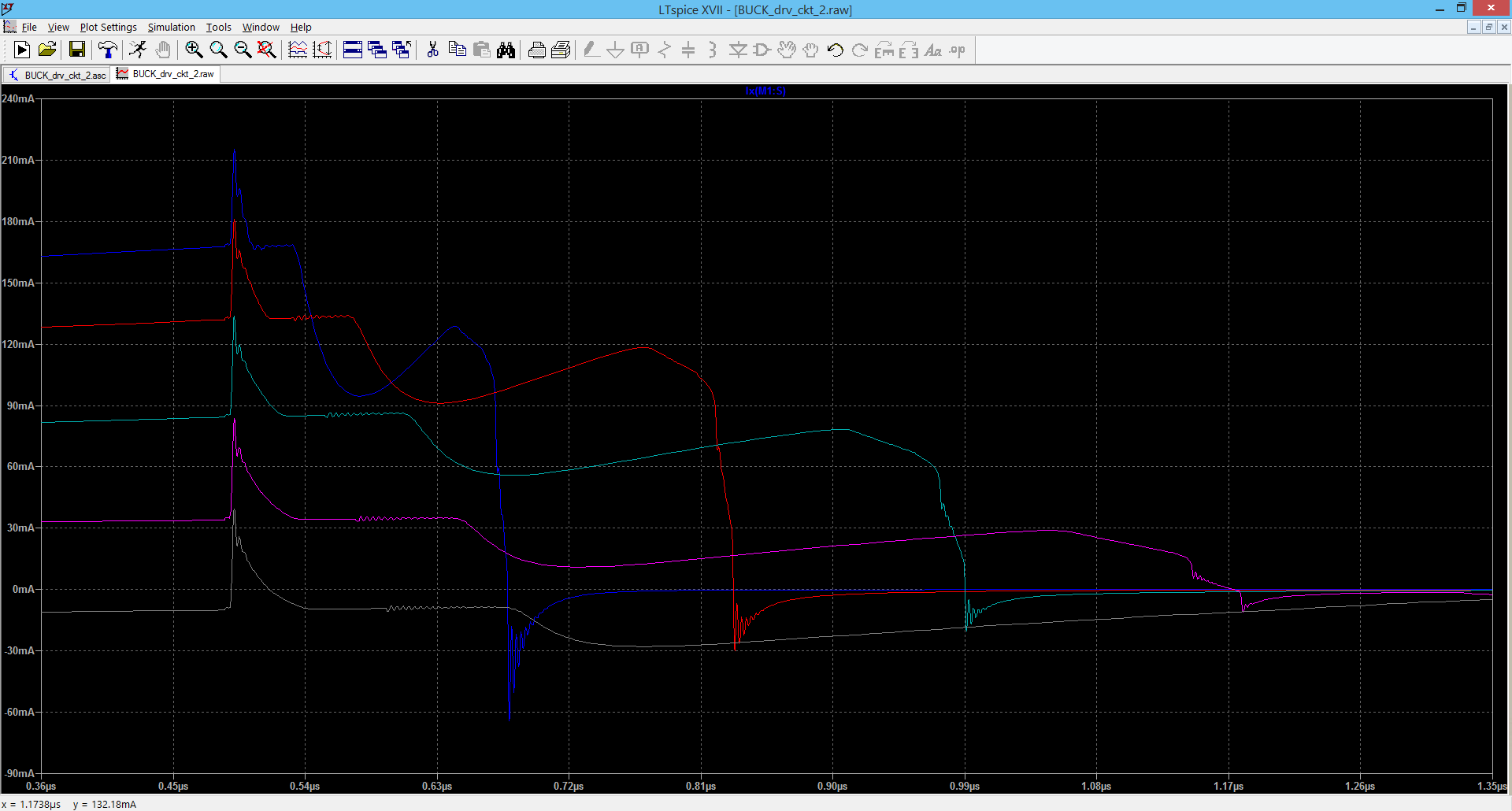
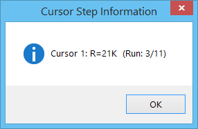
Attach the cursor in the Waveform Viewer window to a specific run (e.g. when using the .STEP statement)
You can attach the cursor from a waveform linked to one run to another by using the up/down keys. By right-clicking on the cursor you can see the step information for that run (see the image below).
Set initial conditions
To set initial conditions use the .IC directive. You can set either node voltages and inductor currents.
Syntax:
.ic [V(<node>)=<voltage>] [I(<inductor>)=<current>]
Example: set the voltage of the node "input" to 5V
.IC V(input)=5
Mathematical & Logical operators list
A list of mathematical operators that can be used in LTspice. source: ltwiki.org
|
Function Name |
Description |
|
abs(x) |
Absolute value of x |
|
acos(x) |
Arc cosine of x |
|
arccos(x) |
Synonym for acos() |
|
acosh(x) |
Arc hyperbolic cosine |
|
asin(x) |
Arc sine |
|
arcsin(x) |
Synonym for sin() |
|
asinh(x) |
Arc hyperbolic sine |
|
atan(x) |
Arc tangent of x |
|
arctan(x) |
Synonym for atan() |
|
atan2(y, x) |
Four quadrant arc tangent of y/x |
|
atanh(x) |
Arc hyperbolic tangent |
|
buf(x) |
1 if x > .5, else 0 |
|
ceil(x) |
Integer equal or greater than x |
|
cos(x) |
Cosine of x |
|
cosh(x) |
Hyperbolic cosine of x |
|
d() |
Finite difference-based derivative |
|
exp(x) |
e to the x |
|
floor(x) |
Integer equal to or less than x |
|
hypot(x,y) |
sqrt(x**2 + y**2) |
|
if(x,y,z) |
If x > .5, then y else z |
|
int(x) |
Convert x to integer |
|
inv(x) |
0. if x > .5, else 1. |
|
limit(x,y,z) |
Intermediate value of x, y, and z |
|
ln(x) |
Natural logarithm of x |
|
log(x) |
Alternate syntax for ln() |
|
log10(x) |
Base 10 logarithm |
|
max(x,y) |
The greater of x or y |
|
min(x,y) |
The smaller of x or y |
|
pow(x,y) |
x**y |
|
pwr(x,y) |
abs(x)**y |
|
pwrs(x,y) |
sgn(x)*abs(x)**y |
|
rand(x) |
Random number between 0 and 1 depending on the integer value of x. |
|
random(x) |
Similar to rand(), but smoother transitions between values. |
|
round(x) |
Nearest integer to x |
|
sgn(x) |
Sign of x |
|
sin(x) |
Sine of x |
|
sinh(x) |
Hyperbolic sine of x |
|
sqrt(x) |
Square root of x |
|
table(x,a,b,c,d,...) |
Interpolate a value for x based on a look-up table given as a set of pairs of points. |
|
tan(x) |
Tangent of x. |
|
tanh(x) |
Hyperbolic tangent of x |
|
u(x) |
Unit step, i.e., 1 if x > 0., else 0. |
|
uramp(x) |
x if x > 0., else 0. |
|
white(x) |
Random number between -0.5 and 0.5 with even smoother transitions between values than random(). |
|
Logic Operator |
Description |
|
& |
Convert the expressions to either side to Boolean, then AND. |
|
| |
Convert the expressions to either side to Boolean, then OR. |
|
^ |
Convert the expressions to either side to Boolean, then XOR. |
|
|
|
|
> |
TRUE if expression on the left is greater than the expression on the right, otherwise FALSE. |
|
< |
TRUE if expression on the left is less than the expression on the right, otherwise FALSE. |
|
>= |
TRUE if expression on the left is less than or equal the expression on the right, otherwise FALSE. |
|
<= |
TRUE if expression on the left is greater than or equal the expression on the right, otherwise FALSE. |
|
|
|
|
+ |
Addition |
|
- |
Subtraction |
|
|
|
|
* |
Multiplication |
|
/ |
Division |
|
|
|
|
** |
Raise left hand side to power of right hand side. |
|
|
|
|
! |
Convert the following expression to Boolean and invert. |
|
|
|
|
@ |
Step selection operator |
|
Constant |
Value |
|
E |
2.7182818284590452354 |
|
Pi |
3.14159265358979323846 |
|
K |
1.3806503e-23 |
|
Q |
1.602176462e-19 |
